
White Papers
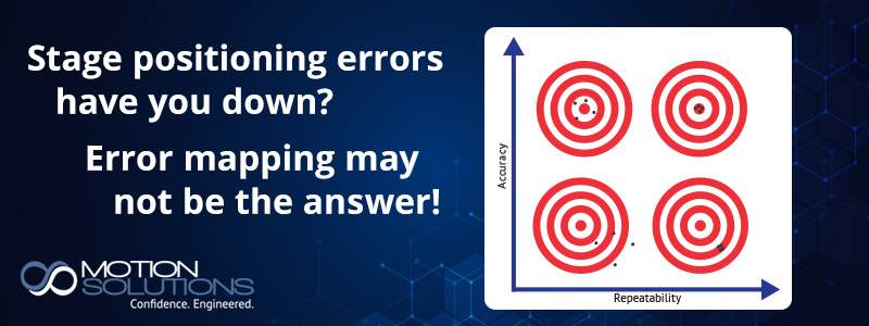
Understanding the Benefits – and Limitations – of Stage Error Mapping
Introduction
Stage error mapping is often presented as a low-cost way to get better performance from a less expensive stage. It’s also suggested as a way to achieve extremely tight accuracy specifications, but the numbers can be misleading. In theory, stage error mapping – measuring absolute positioning error at discrete points – should provide a way to back out that error and improve performance across the complete range of travel. In reality, the benefits are more limited than commonly understood, and the expertise required for execution is greater. For the right application, stage error mapping can be very effective. In many other cases, the results are likely to disappoint. In this white paper, we’ll take a closer look at stage error mapping, reviewing best practices and common pitfalls and misconceptions. Most important, we’ll discuss which classes of applications are best suited to the technology – and which are not.
Accuracy, repeatability, and resolution
We can characterize stage performance using three metrics:
- Accuracy: The difference between the commanded position and the actual position of the load
- Repeatability: The ability of the stage to return to the same position over and over
- Resolution: The smallest increment of the feedback used to control the stage and the smallest mechanical increment of stage movement
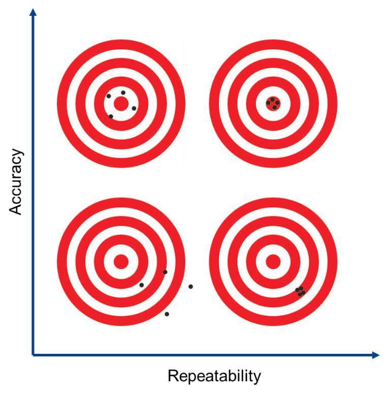
These three quantities should be considered independent. A stage can be repeatable without being accurate, for example (see Figure 1). It can also be accurate without being repeatable. Stage resolution is nominally a function of feedback resolution (for purposes of this white paper, an encoder), but a stage can be high resolution without being either accurate or repeatable.
A variety of error sources affect the accuracy and repeatability of a positioning stage:
- Encoder error – tilt, decentration, etc.
- Motor error – cyclical shaft error
- Signal processing errors
- Stage errors – run out, bearing error, machining errors, improper mounting, etc.
For most applications, these error sources can be controlled to the point that they do not affect overall performance. In the case of applications that require accuracies on the order of a few micrometers or a few arc seconds, however, error sources need to be strictly controlled. One option is to choose higher performance components such as linear motor stages and air bearings. The problem is that the approach increases cost, and every project/product has a budget. This explains the attraction of stage error mapping. To understand why it needs to be used with caution, we have to take a closer look at the process.
What is stage error mapping?
Stage error mapping is the process of measuring the difference between the position reported by the encoder and the actual position of the load at specific sampling points. This data is used to create a lookup table of error per position expressed in encoder counts. The control software uses this for error compensation, extrapolating between points when necessary.
The steps of stage error mapping are as follows:
- Mount the stage on an antivibration table, typically a granite slab, ideally in a ground-floor or even basement location. The stage needs to be installed on an extremely flat surface with no residual stresses that can introduce pitch, roll, or yaw.
- Align the laser interferometer to the stage.
- Command the stage to advance to the desired sampling point using a calculated number of encoder counts. Stop and let the stage settle.
- When the stage is stable, use the laser to measure the difference between commanded position and actual position. Record the data, then command the system to move to the next sampling point and repeat.
- Calculate difference between commanded and actual position at each point and use it to create the error-correction lookup table of encoder counts per position.
- Modify the drive software to extrapolate from the lookup table data to apply the error correction to the command loop.
- Retest after adding the compensation table and repeat multiple times until the desired accuracy is achieved.
The steps are straightforward but how they are performed is crucial to success.
Accurate alignment: Properly aligning the laser interferometer with the stage is essential. Any misalignment of stage relative to the laser can compromise the effectiveness of the map.
Vibration control: At the micrometer/arc second level, even small oscillations can change the measured values. A delivery truck pulling up to the loading dock, a colleague walking down the hallway next to the metrology lab, or even an air current wafting across the room can be problematic, making the use of an antivibration table essential. It’s important to note that not all antivibration tables are created equal, and even the best can only damp perturbation to a certain level.
Temperature stabilization: Thermal expansion and contraction can alter stage behavior. Assemblies should undergo an extended thermal soak prior to data acquisition to ensure stable results. The stage should be mapped at the expected operating temperature.
Multiple runs: A common assumption about stage error mapping is that a single data run is sufficient. Mapping is actually an iterative process in which the data from the first run is used to update the drive commands. Positioning accuracy will be better for the second run but achieving micrometer/arc second accuracies will require three or even four iterations.
By rigorously following the procedures and best practices discussed above, it’s possible to map a stage to achieve high accuracies (see Figure 2). This data plot does not tell the entire story, however.
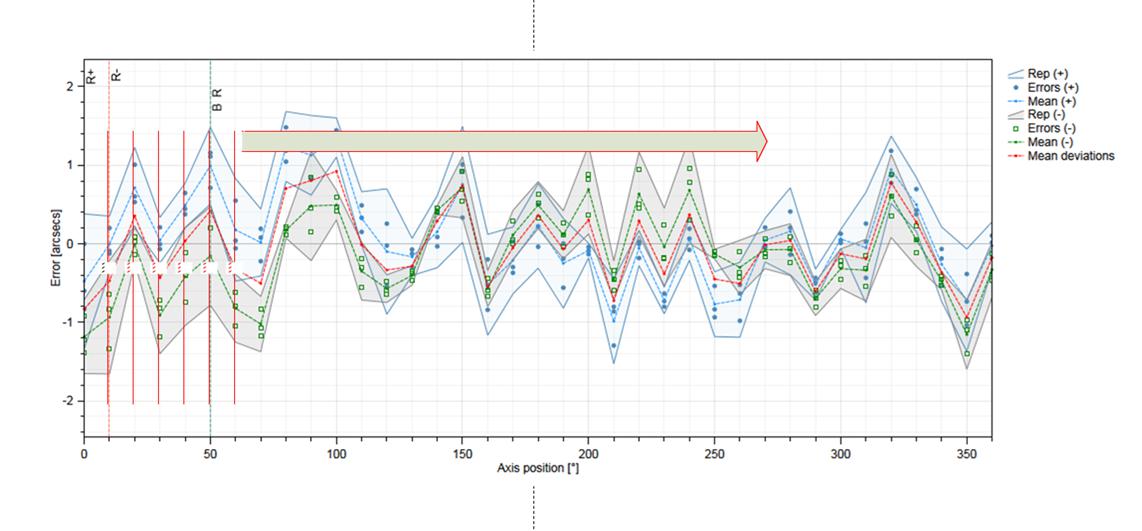
The data appears very promising, yet all too often, that 2 arc second accuracy demonstrated in the metrology lab grows to 20 or 30 arc seconds by the time the stage is deployed in the production environment. OEMs and end-users can be forgiven when they call demanding to know what happened to the stage. Nothing happened to the stage – the problem is rooted in a number of fundamental myths and misconceptions around the capabilities of stage-error mapping.
The issues of stage mapping
Although stage mapping can be effective in certain applications when properly performed, it’s a much more nuanced technique than end users may realize and requires careful attention to detail.
Discrete data can’t necessarily be extrapolated
One of the most common misconceptions about stage error mapping is that it is a continuous process. It’s not, which has profound ramifications. When it’s presented as a possible solution for an application requiring continuous motion, that’s based on the assumption that the error data captured at the sampling points can be extrapolated to reduce error over the full range of travel. This assumption might be true for lower accuracies, but it does not hold for the micrometer/arc second regime. At very high resolutions, positioning error captured at two discrete points tells us very little about performance of the system in between.
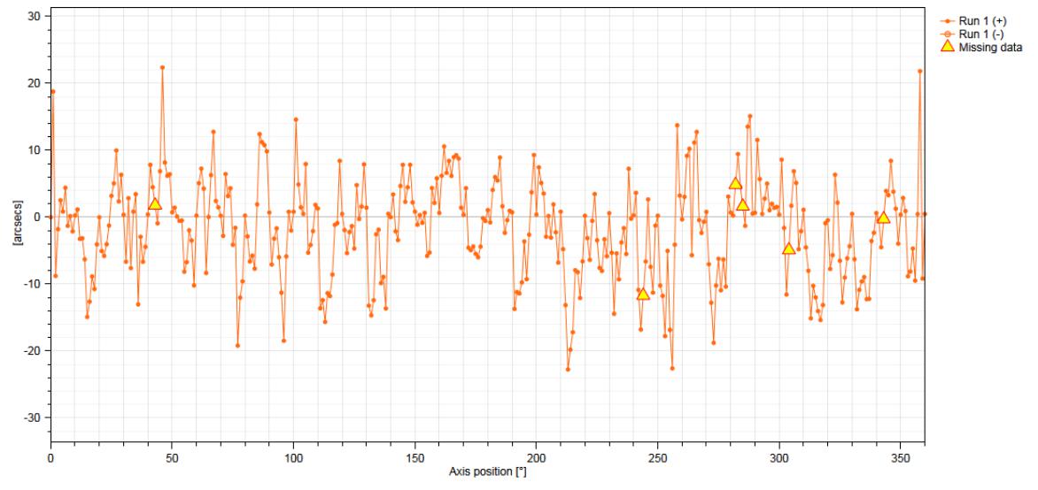
Consider a data run taken on the stage in Figure 2 but based on sampling every 1° rather than every 10°. We see a large, slowly varying error as large as 30 arc seconds that is probably caused by mechanical issues like bearing wobble, machining errors, etc. (see black line, Figure 3).
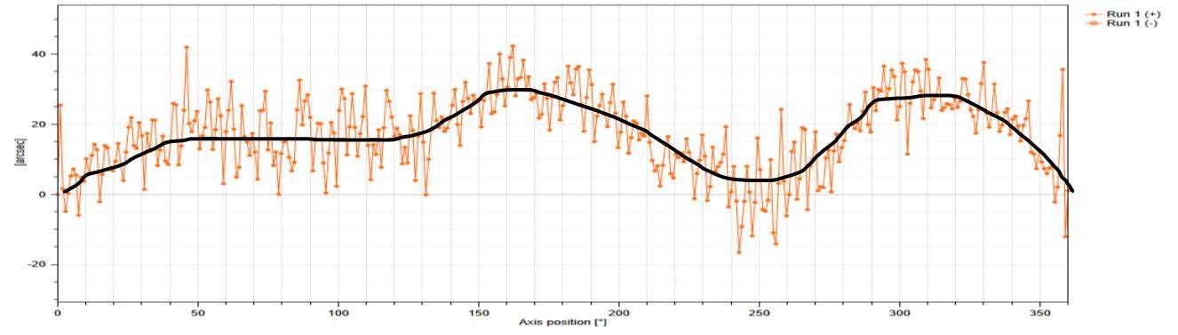
Now, in the case of the low-frequency and repeatable error shown in Figure 3, the assumption about being able to extrapolate between data points holds. We can add correction terms to the control loop to remove the error. That doesn’t necessarily bring us back to the 2 arc second accuracy shown in Figure 2, however. Instead, we have a residual high-frequency error of up to ±30 arc seconds that is most likely the result of small mechanical issues like bearings rotating inside the stage, etc. (see Figure 4)
The data sets at 10° and 1° were taken back to back, without any changes to the set up. If we did another run at 10° increments, we would get the same well-behaved results as for Figure 2. This brings up an important point – stage mapping can be used to repeatably reduce positioning error to micrometer/arc second levels, but only at the points used for mapping. We can’t assume anything about the results outside of those locations. If the homing is off by even a fraction at the customer location, the map will no longer be effective. If the vendor maps the stage at 10°, 20°, 30°, etc. and the actual locations during use change to 15°, 25°, 35°, etc., the map will no longer apply.
Despite these limitations, stage mapping can be very effective in applications like pick and place, for example, or a biotech process that involves moving a probe between two static locations. For continuous applications such as scanning, Z-focus, or genome sequencing, however, stage mapping is unlikely to deliver the level of performance expected.
Increasing sampling frequency boosts accuracy – but also cost
There is a way to address the extrapolation problem, which is to increase sampling frequency. Iterating the error mapping process four times at 1° intervals resulted in a map with accuracies of around 2 arc seconds. Unfortunately, each run also took about two hours, or a full day. Decreasing sampling interval to 0.35° could be used to further improve performance, but now four runs take two days, which becomes extremely expensive. One of the key value propositions of stage mapping is to get improved accuracy from a less expensive stage, but we can clearly reach a point of diminishing returns. That’s a decision that needs to be made on a case-by-case basis, but it should be taken into account during specification.
Conditions change at point of use
We’ve already demonstrated that the effectiveness of stage error mapping for high-accuracy applications is very dependent on whether activities take place at the sampling points. In a perfect world, stage mapping and operation would take place in the same location. In reality, mapping takes place at the factory under ideal conditions, then the stage is packed, shipped, and installed in a new location. With any changes, there is no guarantee that performance will be the same.
- Stage set up and operating conditions when the mapping data is being applied need to be as close as possible to the factory set up when the stage was mapped, with a granite table, tight temperature control, and even an enclosure to block air currents. Customers aren’t necessarily aware of this requirement when they consider stage error mapping. They may lack the resources, or the application may not be compatible with these constraints.
- Mapping at the factory is just the start. Especially if the vendor only supplies input from a single run, the mapping data should be validated after the stage is installed at the customer location. Unless the vendor offers this as a service, the user needs to have a laser interferometer and the in-house expertise to align it with the stage and take data.
Some organizations, including a few of our customers, have both the resources and the need to put these capabilities in place. For the most part, however, this requirement serves as a reminder that stage error mapping may not be the most effective route to micrometer/arc second accuracies.
How to successfully apply stage mapping
Although stage error mapping has its limitations, it can still be very effective for the right application, either by enabling better performance from a less expensive stage or by further improving the performance of a high-end stage.
Talk to your vendor
Be sure that you understand their mapping strategy. What are the conditions during data acquisition? How many points do they use to build the lookup table? Let them know the operating conditions and the stage positions expected during use. If they map the stage at 10°, 20°, etc. and the installed system needs to operate at 15°, 25°, etc., the map will not be as effective. Be sure to share details of the production environment so that they map at the application temperature.
Be realistic
Stage error mapping works best to reduce gross positioning errors. As an example, the effects of screw-pitch error in a ball screw actuator compound with each rotation of the screw. A stage with a 5 mm screw pitch that is actually 5.001 mm could wind up with 300 µm of error by the end of travel. Stage error mapping could be used to reduce this by an order of magnitude. The accuracy level means both that extrapolation applies and that factory mapping will work for the stage as installed by the user.
Improving a ball screw actuator to this level could potentially let it replace a linear motor stage in certain applications. In the micrometer/arc second accuracy regime, it’s difficult to guarantee performance at any location other than the sampling points.
Choose an appropriate application
Particularly for tighter accuracies, the technique should be reserved for positioning at discrete points in applications that do not change. A system that needs to move between two points with extremely high accuracy and repeatability would be ideal for stage mapping. The mapping process for just a handful of points would be fast and economical. Assuming proper mapping and installation at point of use, the stage would perform as expected. That would not be the case for a continuous-scan application like Z focusing.
Another good use case is to correct encoder errors in linear-motor positioners. In these systems, the encoder errors tend to be repeatable and well behaved. The improvements will be small, but in an application requiring the utmost in performance, stage error mapping may be the technique to bring the system to the ultimate level of accuracy required. The caveat is that once again, truly taking advantage of the technique (and the investment) requires validation and optimization of the factory mapping on site.
Pay attention to detail
Install the stage at the application, paying attention to proper mounting and homing. Check for any misalignments that may have been introduced during shipping. If a stacked XY stage loses orthogonality during shipping, for example, the map of the upper stage will no longer apply.
For micrometer/sub arc second accuracies, the lookup table is just the start. You’ll need to set it up with a laser interferometer, first to validate the factory numbers and second to iterate the process to improve performance. Be aware that in a different environment and set up, particularly after shipping, the stage may no longer meet the factory numbers.
If the end goal is truly ultra-high accuracy, be prepared to spend time to achieve the desired performance and understand that the stage is really only likely to meet those numbers at the sampling points.
Conclusion
Stage error mapping can be a useful technique but only when properly applied. It’s very effective to boost the precision of mid-level stages, allowing a ball screw actuator to replace a linear motor for accuracies of tens of micrometers, for example. Limitations arise when it’s applied for applications requiring single-digit micrometer accuracies, however. In these regimes, performance is only guaranteed at the sampling points. This limitation makes the technology appropriate for point-to-point applications but not continuous motion. Users should choose a compatible application and then develop a strategy for proper installation and validation of the stage at point of use. They should talk to their vendors to better understand procedures for mapping and test, and also share application parameters. These measures will make it possible to build a successful system.

About the Author
Bill Lackey is Vice President of Automation.
The Motion Solutions application engineering team has decades of aggregate experience in building precision motion systems. We can help you determine whether stage error mapping can improve your latest project.
Categories
- Case Studies
- Company News
- Customer Focus
- Engineering Insights
- Featured Products
- Industry Perspectives
- nPoint Blog
- Our Take
- Product Spotlight
- Uncategorized