
[EDITOR’S NOTE: For a deeper dive into this topic, see our whitepaper: Understanding the Benefits – and Limitations – of Stage Error Mapping]
Stage-error mapping – measuring absolute positioning error at a specified set of sampling points – has gained a reputation as a method for achieving high accuracy motion control with lower cost equipment. The theory is sound. The problem is that there are a lot of misconceptions around stage-error mapping that can lead to its use in unsuitable applications, with disappointing results. Want to dispel the myths of stage-error mapping and learn how you can use it for maximum benefit? Read on.
Myth #1: Stage error mapping is continuous.
Reality: Data acquisition occurs at discrete sampling points.
During mapping, an external laser interferometer is used to detect the difference between actual position and encoder-derived position at a set of designated sampling points. This data is processed into an error compensation table of counts per position. That table is then used to correct encoder input into the control loop to improve accuracy.
Myth #2: Stage-error mapping only requires one data acquisition run.
Reality: Stage-error mapping is an iterative process, especially for higher accuracies.
The results of the first map are used to modify the encoder input for the second mapping run. The results of the second mapping run will be applied to the third mapping run, and so on. The greater the number of runs, the higher the accuracy – single-digit micrometer or arc second accuracies can require four to six runs.
Myth #3: Discrete data can be extrapolated between sampling points.
Reality: We can’t assume that data at the sampling points tells us anything about performance in between.
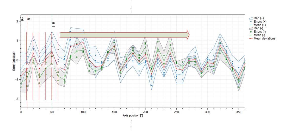
We can map a stage every 10° and perform multiple runs to optimize performance. If we test it at the sampling points, we will see highly repeatable positioning accurate to within a few arc seconds (see Figure 1).
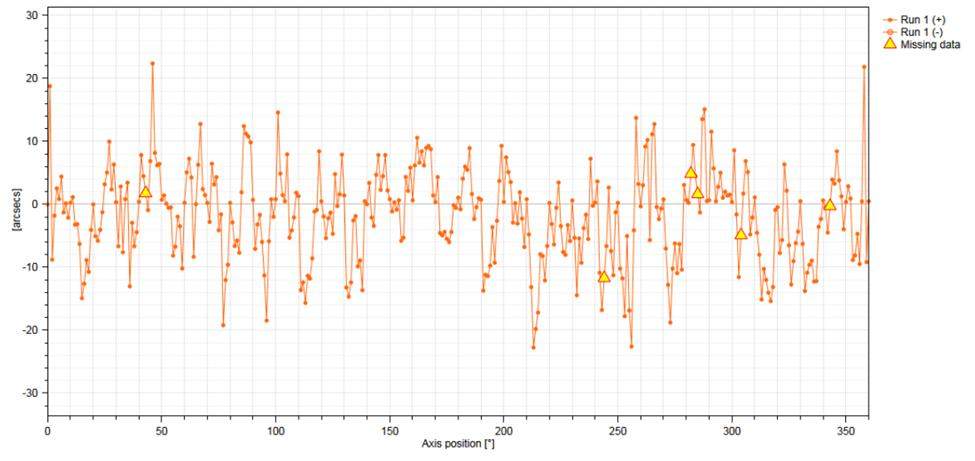
So far, so good. Now, let’s test our mapped system by checking its accuracy every 1° (see Figure 2). Suddenly, our error has grown to ±30 arc seconds. What happened?
Actually, nothing happened. If we check the stage again at the original sampling points, we will still see the same well-behaved performance as in Figure 1. Figure 2 just shows that we can’t make any assumptions about performance in between sampling points. The corollary is that stage-error mapping can be a very effective technique, but only if the stage is used at the sampling points. This limits applications.
Myth #4: Stage mapping is a cheap way to get ultra-high accuracy.
Reality: Not necessarily
Figure 2 shows that when the sampling points are too far apart, large variances can be missed, leading to large errors away from the data acquisition points. Increasing sampling density and the number of mapping runs will improve results. If we take data every 0.36° instead of every 10°, then the error at a position away from the sampling points might be 5 arc seconds rather than 30 arc seconds. The trade-off is cost. Doing one mapping run with sampling points every 10° takes less than 15 minutes. Doing four runs with sampling points every 0.36° increases mapping time to two days. Suddenly, the cost for boosting the accuracy of that bargain stage has gone way up.
Myth #5: Factory performance will carry over to the customer location.
Reality: It depends.
If the stage wasn’t jostled during shipping, if It’s mounted and aligned exactly as it was during factory mapping, and if the accuracy specification is a few tens of microns/arc seconds, then maybe the performance will be similar. Any differences in alignment or homing will prevent the map from correlating to the stage. And if the stage was mapped every 10° starting at zero but the application calls for using it at 15°, 25°, etc., then all bets are off.
Myth #6: Stage-error mapping will solve all of your problems.
Reality: Stage-error mapping can only solve certain problems.
Stage-error mapping can be very effective for moderate corrections – say, improving linear positioning error from 300 µm to 30 µm. This level of performance would allow a ball-screw actuator to be used in place of a linear motor. If the goal is single-digit micrometer/arc second accuracy, then the stage needs to be remapped and optimized at the customer location using a laser interferometer. Even then, it’s really only suitable for point-to-point applications like pick and place or moving a probe between measurement in a biotech instrument. It is not suitable for continuous operations like scanning, z-focus genomics.
When used properly, stage-error mapping can be a powerful technique for getting effective performance from more economical components. The key is to watch out for the myths that can lead to disappointing performance. Start with an appropriate application. Talk with your vendor to understand their mapping process. Follow best practices for installing the stage. Most important, remember that accuracy is only dependable for a properly mounted stage and only at the sampling points.
Find out whether stage-error mapping can improve your next project. Reach out to our team of experts at Motion Solutions.

About the Author
Bill Lackey is Vice President of Automation.